Process mode is the workspace for reviewing, reprocessing, saving, and exporting previously recorded Vimotis data. Use this mode when an acquisition file already exists and you need to inspect signals, adjust processing settings, add markers, export data, or compare channels across files.
Process mode supports:
- loading recorded
.h5or.hdf5files, - reviewing wave-speed, calibrated-load, analog, correlation, and foot-contact views,
- updating processing parameters and calibration data,
- adding marker points to selected channels,
- saving reprocessed results back into the loaded HDF5 file,
- exporting CSV outputs and figures,
- running batch reprocess or export workflows, and
- comparing channels across files in the Evaluation window.
Always post-process tensiometer data before detailed analysis or exporting. The processing algorithms which allow for live data display are less robust than those used to post-process the data.
Menus and Dialogs
When Process mode is active, these unique process mode menu actions are available:
- File > Load: load a Vimotis HDF5 file.
- File > Save: save reprocessed results into the loaded HDF5 file.
- File > Export: open the CSV export dialog.
- File > Batch: open the Batch Process workflow.
- Edit > Calibration: open calibration settings for Process mode.
- Edit > Parameters: open normal processing parameters.
- Evaluate > Open: open the Evaluation window.
Loading Data and Sources
The current implementation loads HDF5 files with .h5 or .hdf5 extensions. If a file contains both live and reprocessed results, the user will be prompted with a pop-up to choose whether they wish to load Live data (as collected and viewed in real-time) or Reprocessed (post-processed and saved data).
Additionally, if a file is already loaded in the workspace, and the user chooses to load Live data, a dialog will pop up with options Keep Current or Reset Defaults.
Keep Currentallows the user to keep the processing parameters they set/loaded from the previous file in the workspace. Note that to apply these parameters to the new file, the user will need to runReprocess All.Reset Defaultsresets the workspace parameters to the defaul reprocessing parameters.
Save Data
Reprocessed data is not saved by default to prevent loss of desired data when viewing or experimenting with different processing parameters. To save reprocessed data, choose File > Save. Reprocessed data is stored in the same file as the Live data. Only one set of Reprocessed data can be saved per file; any future saved reprocessing will overwrite old Reprocessed data. Once Reprocessed data has been saved, it may be chosen for viewing/reprocessing when loading that file in the future.
Workspace and Plot Controls
The main Process workspace includes a left-side channel selection area and plot tabs for reviewing the loaded file.
- Switch between
Wave SpeedandCalibrated Loadusing the dropdown in the upper-right of the main plot tab. - Plot items can be hidden/revealed by clicking on the legend entry to toggle visibility.
- The x- and y-axis zoom is controlled by clicking and dragging in the direction and over the region of interest. Double-click to reset the axes.
Channel Select
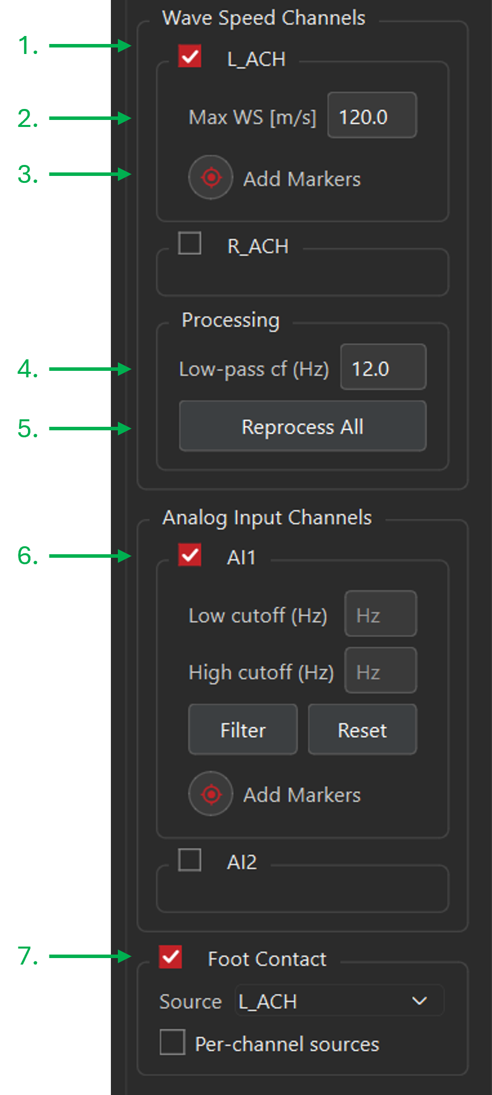
The left-side channel control area is used to choose which channels are visible and which channel is active for marker editing.
- Channel check boxes determine which wave-speed and analog signals are visible.
- The Add Markers controls choose the active wave-speed or analog channel for marker editing.
- Sets the low-pass filter cutoff used for wave-speed smoothing. The filter is a zero-phase second order Butterworth filter with a maximum cutoff of 50Hz (Nyquist).
- The
Reprocess Allcontrol recalculates selected wave-speed outputs with the current processing settings. - Analog data aquired on auxiliary AI ports are displayed on separate axes below the load plot. Optional low/high/bandpass filtering (2nd order Butterworth) can be applied to these data on a per-channel basis.
- For relevant datasets, foot contacts can be applied. These are estimated using alternative processing of the raw tensiometer data and should only be used as estimates.
Correlation Image
The core data processing algorithm computes a wave speed based on a changing time delay (Δt). The time delay represents wave travel time between the two sensor contacts and is found using cross-correlation based algorithm. This time delay (shown in red), overlayed on a heatmap representation of the two sensor contact signal correlations can be viewed in the Correlation tab.
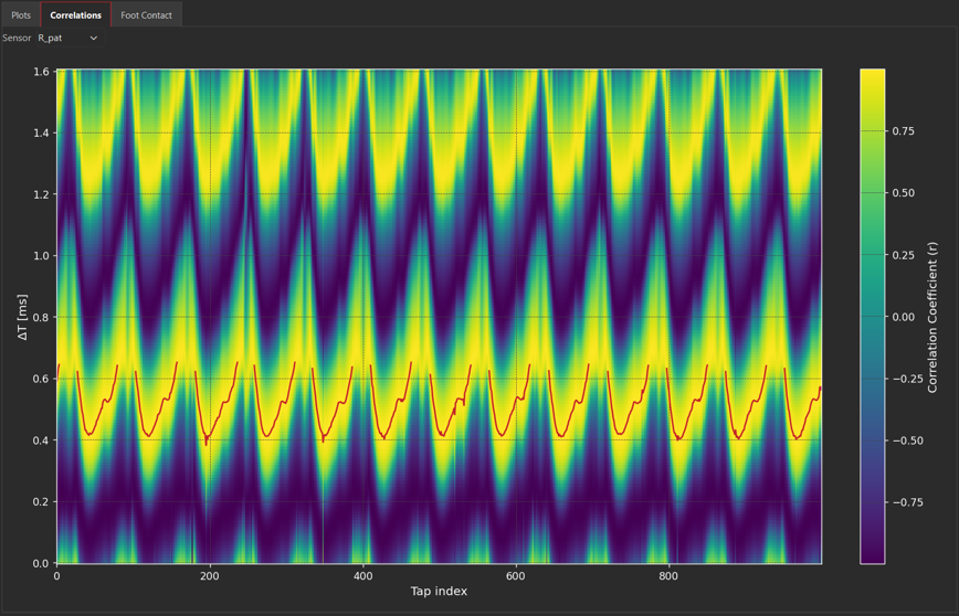
The x-axis indicates the tap index, or the index of the excited wave. The tap rate is 100 Hz, so the number of indices should be 100x the duration of the collection in seconds. The y-axis indicates the full length of possible time delays (Δt) values for a given tap n. The heatmap indicates the correlation strength at each possible time delay, with the final time delay following the peak values in the correlation image. Since the waves are oscillatory, multiple peaks can be observed, and the processing algorithm determines the appropriate peak trace from which to compute wave speed and load. Gaps indicate data that were excluded by the quality gate settings. For tap indices without any high correlation coefficients (yellow in the plot), shape similarity between the upstream and downstream signals is low, so confidence in the Δt value is low.
Foot Contact
For gait tasks, foot contacts may be optionally estimated. To enable, check the foot contacts box in the left channel bar. The channel source for the foot contacts may be selected from the dropdown, or each channel may be assigned a foot contact source if Per-Channel Sources is selected.
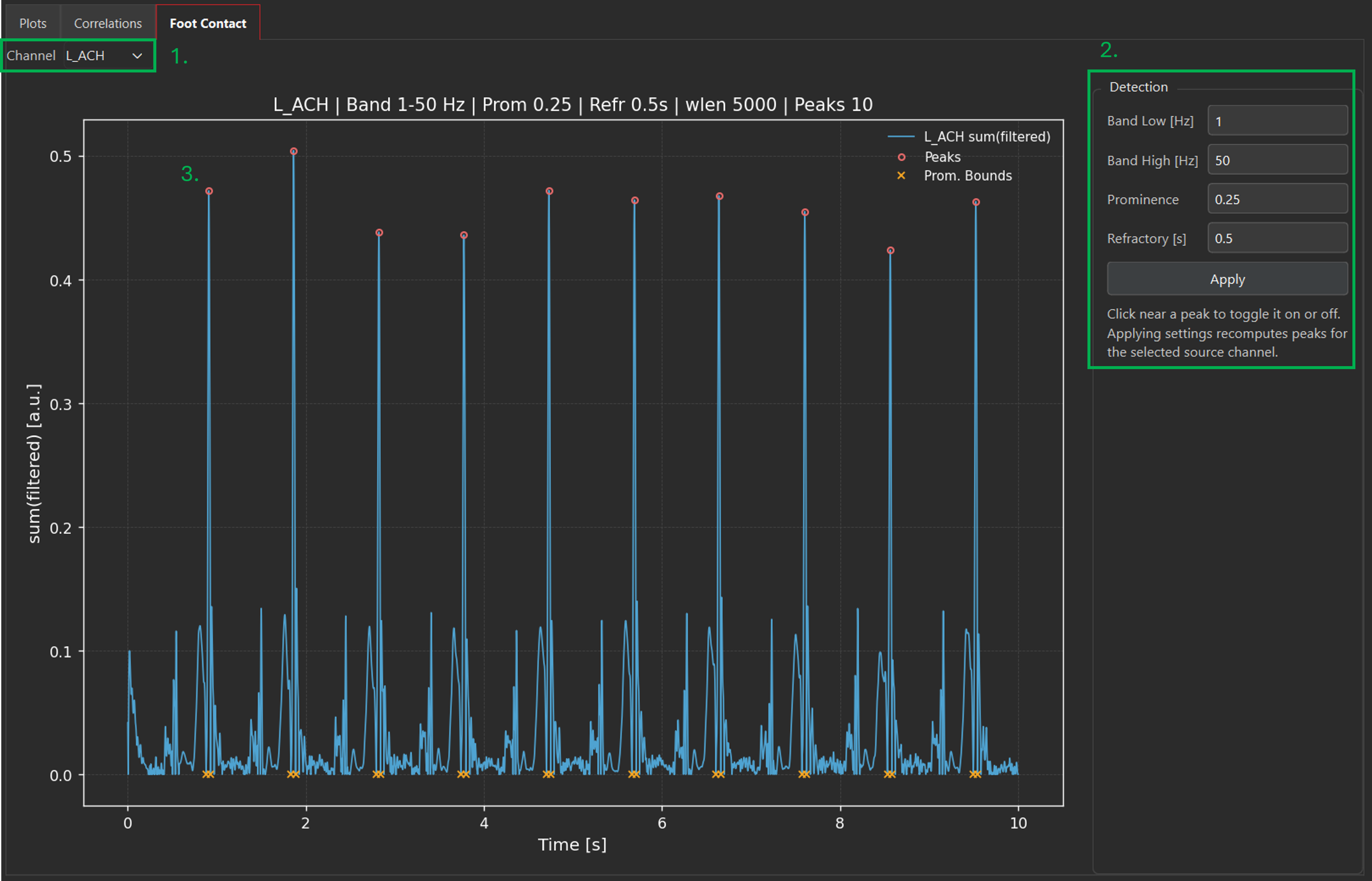
- Choose which channel is shown for foot contact estimation from the dropdown.
The foot contact detection uses features in an accelerometer signal to estimate ground impact. Depending on the task and sensor location, the parameters to isolate foot contact features may require optimization. The available parameters are:
- Band Low/High [Hz]: Bandpass filter cutoffs.
- Prominence: Amplitude of feature peak relative to local minima.
- Refractory [s]: Minimum permitted time between foot contact events. For example, during high-cadence running, the time between events will be much shorter than walking, so a shorter refractory should be used.
- Foot contact event detection may be edited diretly by single-clicking on peaks to add or remove them. Recomputing foot contacts after changing parameters will remove manually edited events.
- Switch between point interaction and zoom mode using the respective buttons.
Data Markers
Markers may be added per-channel to denote timing or specific features of interest. These are exported in a column vector time-synced with the rest of the data for external proecessing. Note that in marker mode, the standard x/y zoom interaction is toggled with the associated button.
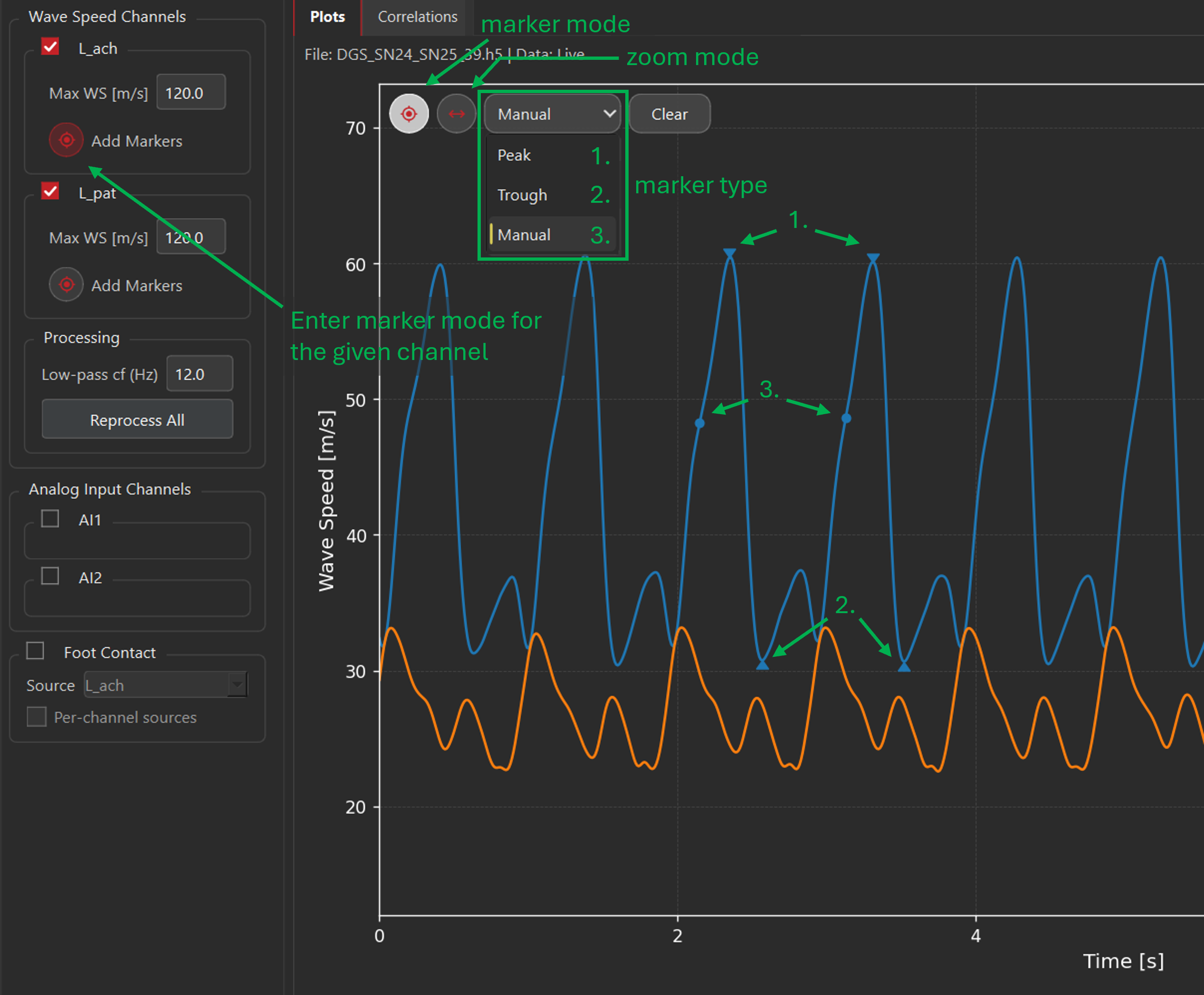
Markers are saved with reprocessed results and included in CSV exports when the Markers export option is selected.
Process Parameters Dialog
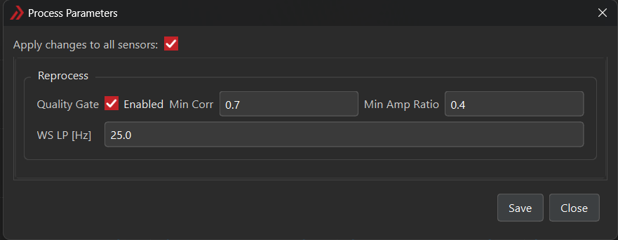
The Process Parameters window supports per-sensor editing of processing settings.
| Setting | Description |
|---|---|
| Apply changes to all sensors | Applies the visible parameter changes across all tensiometer channels. Uncheck to change individual channel settings independently. |
| Tensiometer tabs | Select the sensor whose processing settings are being reviewed or edited. These are only enabled when Apply changes to all sensors is disabled. |
| Quality Gate | The Quality Gate is used to mask data in which there is low confidence based on two parameters. Min Corr is the minimum allowable cross correlation coefficient found when computing the wave travel time (Δt) between the two sensor contacts; it is a measure of distortion, or lack thereof, in the signal as it is transmitted from contact 1 to contact 2. Too much distortion between the signals lowers confidence in the computed Δt (see Correlation Image and Section 7.4 of the Product Manual). Min Amp Ratio is the minimum ratio between the maximum amplitude of the signal measured at contact 2 divided by contact 1; it represents how well the signal is being transmitted through the tendon. |
Use Reprocess All in the main app window after changing parameters when the loaded data should be recalculated with the updated settings.
Calibration Workspace
The post-process calibration dialog mirrors the acquisition calibration dialog, not including the ability to capture calibration data. Here, any parameters may be updated and the calibration recomputed. See Acquire Mode: Calibration for details on individual settings.
When data are captured with an active calibration, the data files share an identifier with the calibration archive file which allows them to stay linked as long as the calibration and data remain in the same file directory. If a calibration file stored in a different directory needs to be applied to a data file, the calibration file can be loaded in the calibration workspace.
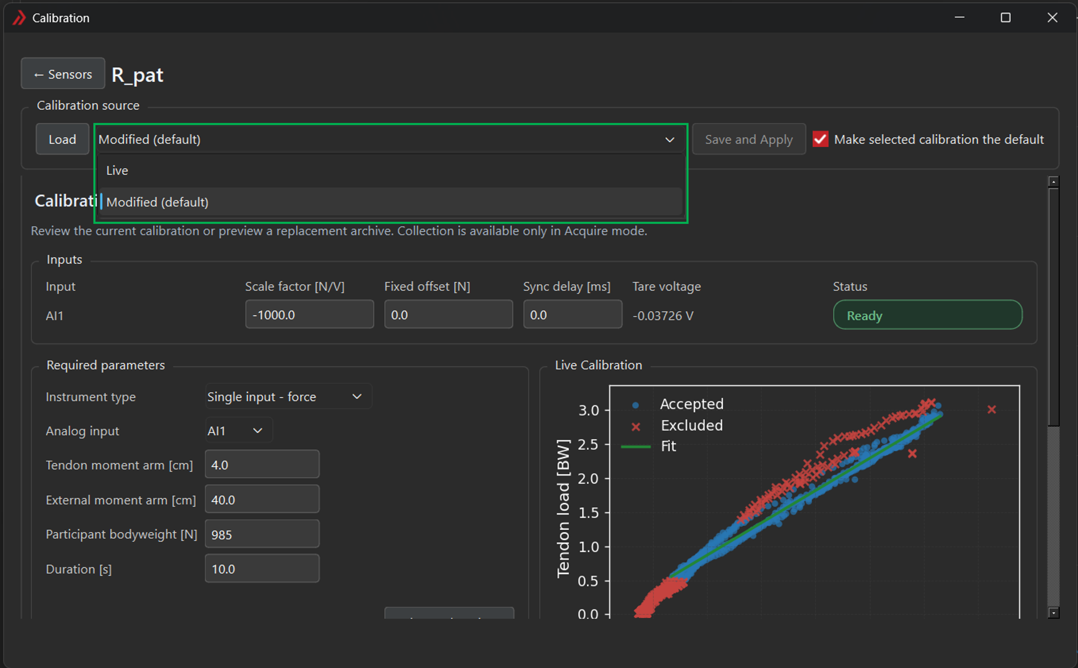
If calibration parameters are changed and the new fit is computed and applied in Process mode, the results are saved under a parallel archive labeled 'Modified'. This archive is stored along side the 'Live' archive in the same file and does not overwrite the settings saved during the original acquisition.
The user may choose which archive (Live or Modified) is loaded by default, and the Modified archive may be edited and recomputed, but any future changes to parameters will overwrite the saved Modified parameters.
The calibration workspace can be accessed for individually loaded trials from Edit > Calibration or in the batch wizard during Step 2. Note that any changes to the calibration archive will apply those changes for all data files linked to that archive.
CSV Export Dialog
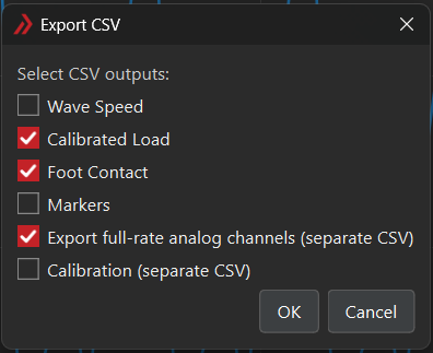
File > Export opens the CSV export dialog.
| Option | Description |
|---|---|
| Wave speed | Exports wave-speed data from the selected source. |
| Calibrated load | Exports calibrated-load data when calibration data are available. |
| Foot contact | Exports foot-contact data when available or generated. |
| Markers | Includes saved marker locations in the export. |
| Full-rate analog channels | Writes full-rate analog data to a separate CSV. |
| Calibration | Writes calibration data to a separate calibration CSV. |
The application warns before overwriting existing CSV files.
Batch Process Dialog
File > Batch opens a guided workflow that can run in two modes: Reprocess Files and Export Existing CSV Only. Export Existing CSV Only is intended for use when only the export function is required. The workflow is organized into four steps:
Select Files: choose a source folder and move files into the
Files To ReprocessorFiles To Exportlist.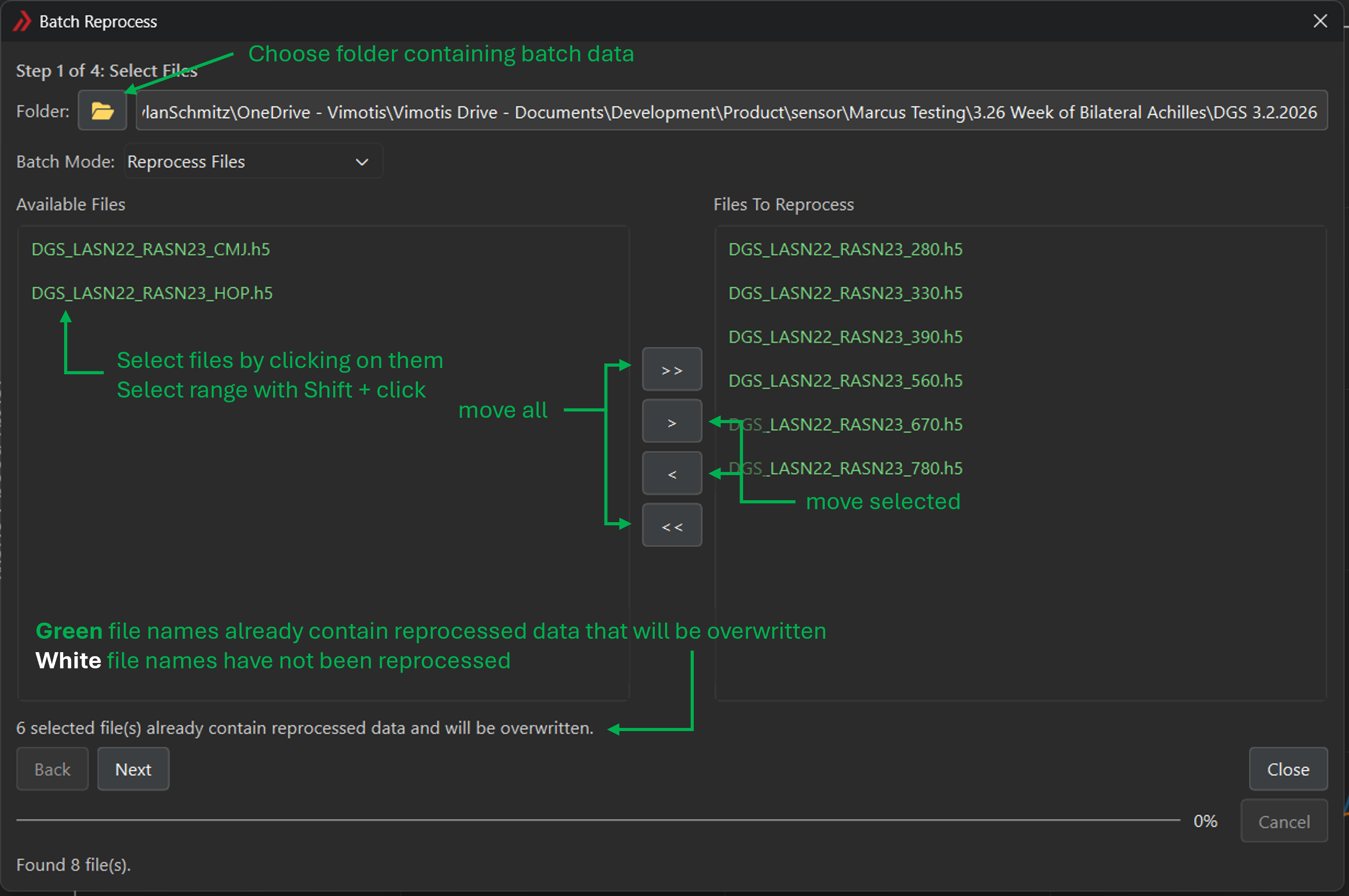
Figure 8: Batch Process file-selection step used to choose source files. Confirm Parameters: review or seed processing parameters when reprocessing. This step is skipped in
Export Existing CSV Onlymode.Option Description Use Defaults Reprocesses using standard settings. Seed From File Applies the processing parameters from the selected file to all files. May choose between Live and Reprocessed if available. Seed From Workspace Applies the processing parameters from the workspace. The intended use case is: load an individual file to the workspace. Modify processing parameters until desired results are achieved. Run the batch wizard and apply workspace parameters to batch. 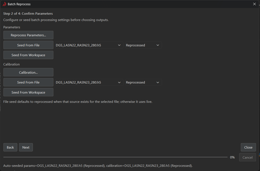
Figure 9: Batch Process file-selection step used to choose source files.
The linked calibration file will be loaded automatically if it is in the same folder as the data files being processed. If not, the file can be manually loaded. The calibration settings can be viewed and edited/saved by launching the calibration workspace with View Parameters (see Calibration Workspace). Important: only files which share a calibration archive should be batch processed together to prevent mismatching.
Save and Export: choose the batch mode, data source, CSV outputs, summary plots, and foot-contact options.
These options mirror those in the Export dialog.
Additionally, choose whether to compute foot contacts for the batch files. As with the workspace Foot Contact options, these can be sourced from a single channel for all channels (e.g. all sensors/signals associated with the right leg), or applied independently to each channel (e.g. bilateral measurements).
An optional summary plot may be selected to show all processed data after the batch runs.
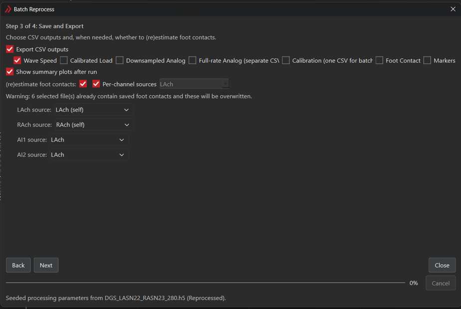
Figure 10: Batch Process file-selection step used to choose source files. - Review and Run: confirm the selected files, parameter/calibration sources, and export options before starting.
Always review the summary before running the batch, as previously reprocessed data in batch files will be overwritten. Once you have confirmed the details, choose Run Reprocess. The progress bar at the bottom of the wizard will show the batch progress.
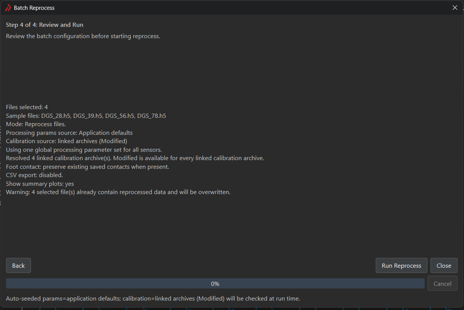
Normal Output
When a file is saved from Process mode, the application writes reprocessed outputs back into the loaded HDF5 file.
Current saved outputs can include:
- reprocessed wave-speed data under the reprocessed wave-speed result path,
- processing parameters,
- foot-contact vectors and related debug data when generated, and
- marker data.
CSV filenames include the loaded file stem and the selected data-source token:
- Main CSV:
{stem}_{source_token}_postprocess.csv - Full-rate analog CSV:
{stem}_{source_token}_postprocess_full_ai.csv
If reprocessed data already exist in the file, the user is prompted before it is overwritten.
Evaluation Window
The Evaluation window can be accessed via the Evaluate > Open menu. This tool is intended to allow for quick comparisons of data across one or more files and should not be a substitute for a more thorough data processing pipeline.
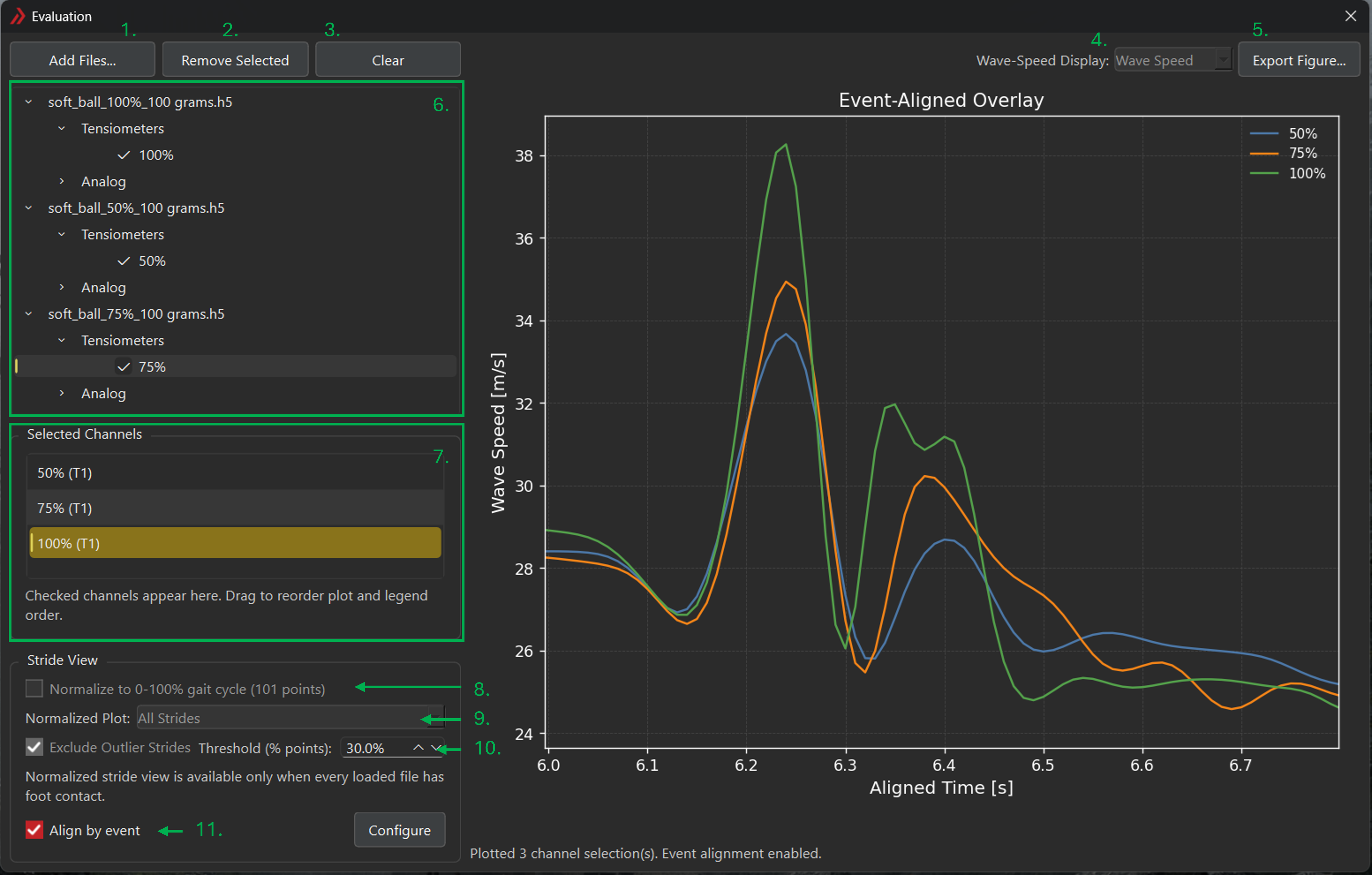
Add Files...loads one or more HDF5 files into the comparison set.Remove Selectedremoves highlighted files from the comparison set.Clearremoves all loaded files.Displaydropdown toggles between wave speed an load.Export Figureopens the Export Figure dialog.
File/channel tree
- Check/uncheck boxes to add/remove channels on the plot. Double-click on a channel name to assign an alias to the channel. This alias does not change the underlying data but can be useful to clarify the plot legend.
Analog channels are plotted on a separate axis below the wave speed / load axis.
Selected Channels
- Shows the active comparison channels. Drag and drop items in this list to reorder the plot entries and legend.
Stride View
- If foot contacts have been computed for the loaded files, checking the box will time-normalize each stride to 0-100% gait cycle.
- Strides may be plotted in aggregate (all strides not eliminated by the outlier threshold) or as an ensemble average (+/-1SD).
- Based on leave-one-out analyses at each point in the gait cycle, strides in which the number of outlier points exceeds the threshold (default 30%) are excluded from the plot and ensemble average.
Align by event is an alternative to foot-contact based alignment for non-repetitive tasks (e.g. jumping, pitching). Choose
Configureto launch the Align by Event wizard.Configure event alignment
- Alignment: choose
One PointorTwo Points.One Pointidentifies a single point in each channel and translates all traces such that the selected point in each channel is aligned.Two Pointsboth translates and linearly warps each channel so that both selected points are aligned across channels. - Point Type: options are
Peak,Trough, orManual.PeakandTroughwill identify the nearest feature of matching type when selecting.Manualwill place the point at the location clicked. - When plotting multiple channels from the same file, you may choose to apply the alignment point(s) across those channels or set them independently.
- Alignment: choose
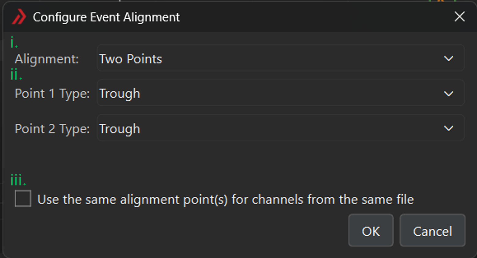
Figure 12: Align by Event wizard, configure event alignment. Choose points
For each channel, select the desired alignment point(s), using
Nextto proceed through each plot. To adjust a selected point, use the upper-left dropdown to choose which point you want to adjust, then reselct the correct location. Once all points have been selected for all channels, chooseFinish
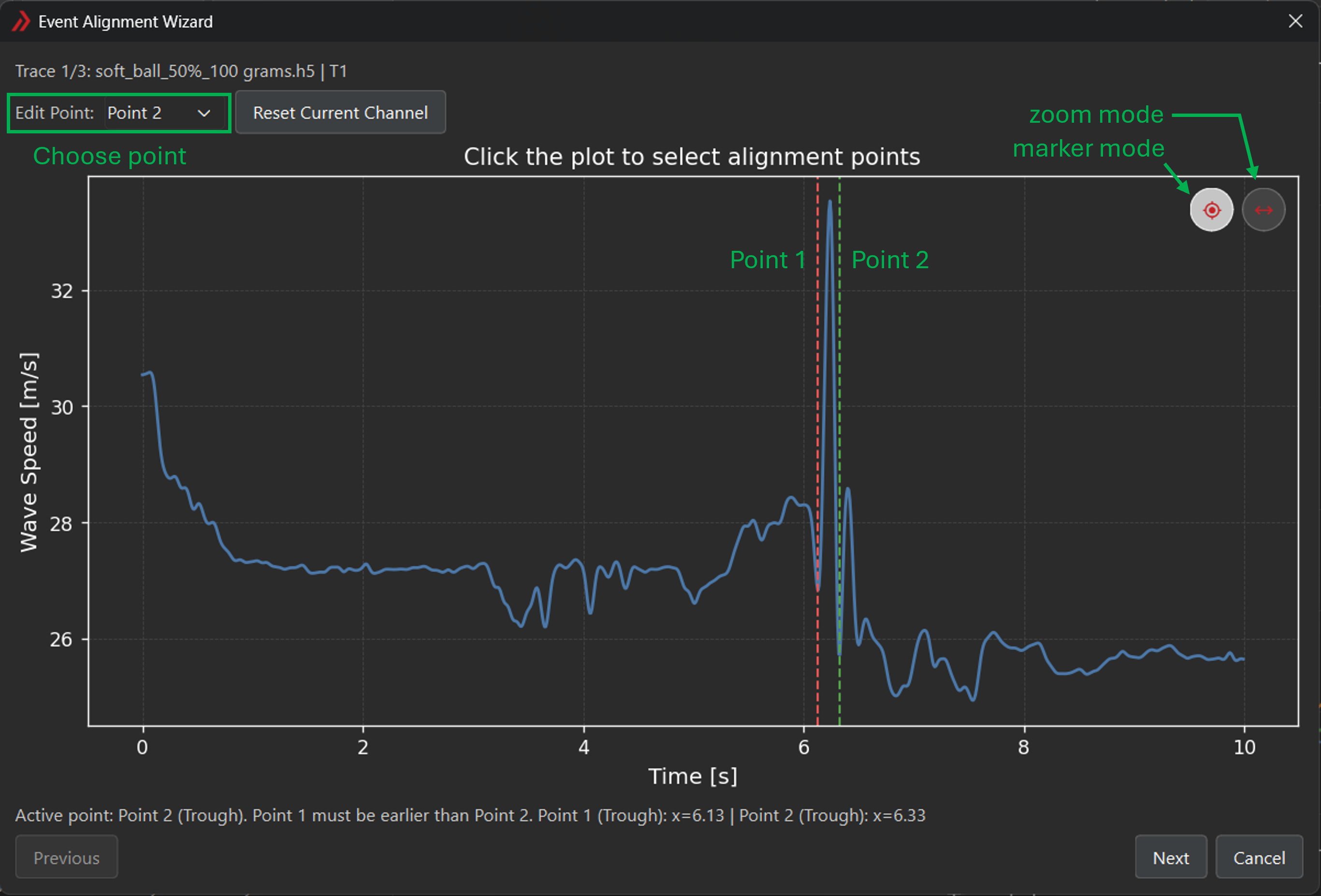
Figure 13: Align by Event wizard, choose points - Once the pipeline is complete, the checkbox will be enabled to toggle the event alignment.
Export Evaluation Figure Dialog
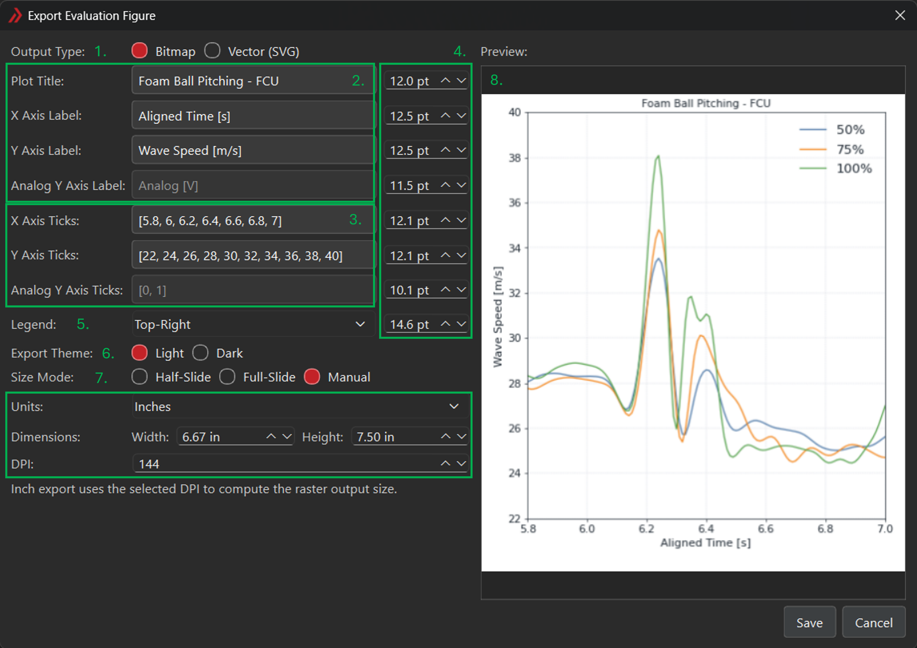
The Export Evaluation Figure dialog is used to configure plot output before saving a comparison figure.
- Output type: Selects
BitmaporVector (SVG). - Plot title and axis labels: Sets the title and axis text used in the exported figure. These are applied only in the export preview and will not impact the main Evaluate window plot.
- Axis ticks: Set location of axis ticks. To auto-fill an evenly spaced range, use the syntax [low:step:high].
- Font sizes: Independently control font size for title, labels, and legend.
- Legend placement: Sets where the legend appears in the exported figure.
- Export theme: Selects the visual color theme used for output,
DarkorLight Size preset: Options for exported figure size, selects
Half-Slide,Full-Slide, orManual.Half-SlideandFull-Slideare based on standard Powerpoint slide dimensions. IfManualis chosen, additional options are exposed:- Units: Selects pixels, millimeters, or inches.
- Dimensions: Width and height of exported figure in specified units.
- DPI: Controls bitmap export resolution (if Output type is
Bitmap)
- Preview: Shows a live preview of the configured figure (resolution will be lower than exported image).
Vector export saves SVG. Bitmap export supports PNG and JPEG.